The sense of hearing provides us with the possibility to explore and interact with our surrounding environment. Examples of this interaction are the ability to localise a sound object or to obtain information about its identity (Osses2018). While these examples are very basic tasks in our everyday lives, the mechanism behind hearing, the processing in the auditory system, is of high complexity. The auditory system has been studied since old times, first hypothesising how sounds were processed, as done by Pythagoras in the sixth century B.C. Much later, evidence started to be collected, mainly as a result from experiments with animals and human bodies, as reported by Andreas Vesalius and Bartolomeo Eustachi in the 16^th century, and the research on the functionality of the cochlea in the inner ear by Philipp Meckel (17^th century), Alfonso Corti (19^th century), and von Bekesy (20^th century) (Stevens1968). In the last decades, research into the functionality of the auditory processes has been strongly supported by the development and evaluation of computational models that are assumed to reflect fundamental aspects of the auditory system (see, e.g., Osses2022).

The current article represents a brief introduction to the auditory system and hearing mechanisms. The focus here is not much on specific listening situations but rather on the specific parts of the auditory system and their rough approximations of the underlying processes. More in depth explanations can be found elsewhere (e.g., Moore2013).

The auditory system consists of a mechanical part and a neural part. The mechanical part starts with the pinnae, our ears, that drive the sounds into the ear canal. After several transformations the sounds are converted from air pressure variations into electric impulses represented as neural patterns, with the first train of pulses originating in the auditory nerve and being conveyed to higher brain stages. The mechanical part consists of the outer ear, the middle ear, and the inner ear and there is quite some consensus in the role and in how these stages operate in the auditory system. The neural part comprises the connectivity and involved functional mechanisms that transmit firing patterns in the auditory nerve, though the central nervous system to the brain (e.g., Kohlrausch2013). Unfortunately, the neural processes lack a consensus in the way in which sounds are exactly further processed, especially at the level of the auditory cortex where cognitive or “top-down” aspects start to interact with the signal-based or “bottom-up” information coming from the auditory processing in earlier stages.

The mechanical and neural parts are schematised in Figure 1.

Incoming sounds are pressure variations with respect to the atmospheric pressure and are, therefore, expressed in units of pressure, Pascals (Pa). These pressure variations vary strongly in time moving back and forth from positive to negative amplitudes. The ear is an organ that reacts to a large range of amplitudes, namely between the audibility threshold of 2 x 10^-5 Pa and the pain threshold at around 10² Pa. Because of this large range (about 7 decades, or a pain threshold that is 5 million times the audibility threshold), sound pressure amplitudes are more conveniently expressed in decibels, relative to p₀=2 x 10^-5 Pa, in a way that the Pascal scale is compressed to a range between 0 and 134 decibels (dB). Actually, when referencing the pressure variations to this value of p₀, a common practice in physiology is to add the suffix sound pressure level, such that the amplitudes are expressed in dB SPL. In acoustics, this is not always the case, as it is often assumed that when the 0 dB reference is not specified, the standard p₀ reference is assumed.

Because of the usefulness of adopting a logarithmic scale to express incoming amplitudes, it is often said that the auditory system acts as a compressor. The time-varying amplitudes or waveforms (see Figure 2) are, however, often expressed in Pascals, whereas the overall level or root-mean-square (RMS) value of sound is expressed in dB SPL.

A representation of an incoming sound or waveform, the sentence “It will not be too expensive, surely she said” is presented in Figure 2. This waveform has an RMS value of 73.6 dB. This same sentence is used in subsequent sections to exemplify the process introduced by each part of the auditory system.

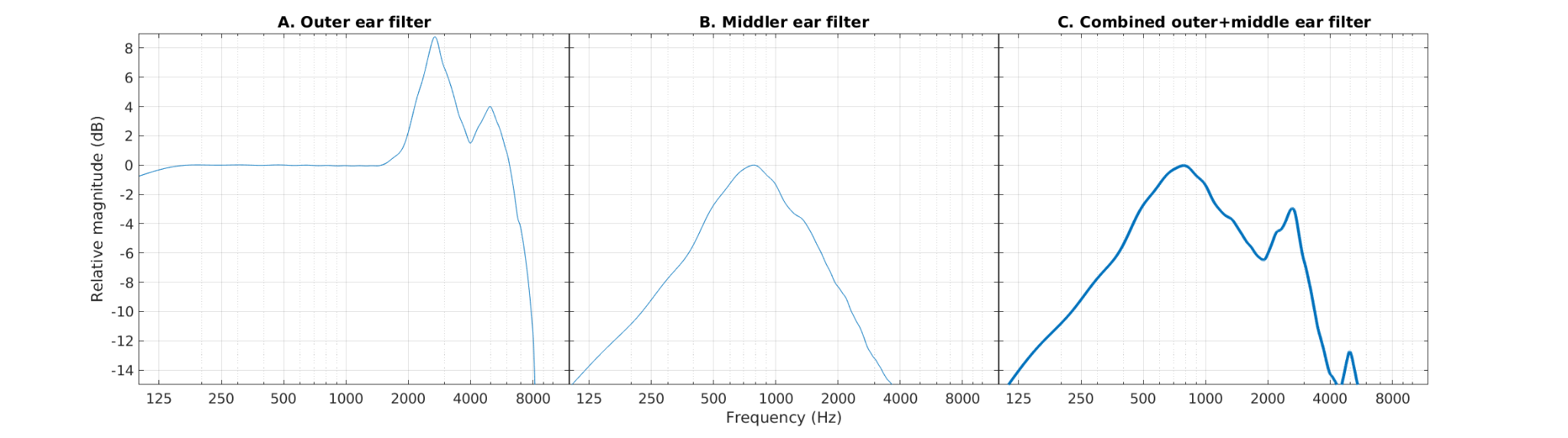
The listener’s head, torso, and pinna shape the incoming sounds, acting as filters that emphasise and de-emphasise specific frequencies. One of the most emphasised frequency regions is located at around 3200 Hz as it corresponds to the resonance of the ear canal.

The combined effects of the head, torso, and pinna are often approximated using the so-called head-related transfer functions (HRTFs) (Moller1995, JAES). This process is often approximated as a linear filter. Its effect is shown in Figure 3. The waveform is not visibly (to the naked eye) different from the original sentence. The presented approximation results from applying a filter as depicted in Figure 4A.

The signal at the end of this processing stage represents the ear canal pressure at the level of the tympanic membrane and is still expressed in Pascals.

The waveform at the level of the tympanic membrane has amplitudes that are too weak. The middle ear acts as an amplifier and actually as an impedance matcher between the air pressure variations coming from the outer ear and the fluid oscillations that will be produced in the inner ear. The middle ear starts with the tympanic membrane and ends with the oval window, which are connected by three bones or ossicles, the malleus (PT: martelo), the incus (PT: bigorna), and the stapes (PT: estribo). The first two bones were discovered by Andreas Vesalius in 1543 and allowed to discard completely the erroneous old theory that the auditory system was a system filled in by air.

In practice, the middle ear introduces a bandpass characteristic centred at about 800 Hz, with a gain in this range of about 20 dB (e.g., Puria 1997, Puria2020-AT) and slopes of 6 (or -6) dB/octave for the lower (or higher) skirts of the filter. The 20-dB gain needs to be interpreted with care, as the waveforms at the end of the middle ear (oval window), are no longer expressed in Pascals, representing either the stapes displacement (m) or stapes velocity (m/s). In the example we are providing, a 0-dB gain in the bandpass was applied. The amplitudes of the waveform shown in Figure 5 are thus expressed in arbitrary units. The bandpass characteristic of the middle ear filter alone, our approximation here, is shown in Figure 4B, whereas the combined frequency response of the approximation of outer and middle ear filters are shown in Figure 4C.

The inner ear or cochlea is shaped like a spiral that is filled by fluids and enclosed by rigid walls. The basilar membrane is one of the structures of the inner ear and its movement is elicited by the incoming sounds. The cochlea starts near the oval window. This side is known as base. The cochlea extends up to the apex, where there is a small opening called helicotrema. The length of the cochlea is approximately 35 mm. The basilar membrane presents a maximum oscillation that depends on the frequency of the stimulation, with sounds of high frequency being related to gradually more basal locations and, conversely, sounds of low frequency being related to more apical locations. The frequency to position mapping along the cochlea is schematised in Figure 6.

In other words, different sections of the cochlea are sensitive to different frequency ranges. For this reason, a first approximation to the inner ear processing is as a filter bank. Perceptual (psychoacoustic) experiments have shed light into the width of such a set of filters (Zwicker1961, Moore1983), that have been named critical bands. A general agreement is that the critical bands are wider towards higher frequencies. A well accepted resolution is defined using the equivalent rectangular bandwidth scale (ERB, Moore1983). Using a filter bank based on an ERB spacing, our test sentence decomposed in a number of selected bands is shown in Fig. 7.

The inner ear processing is however much more complex than the filtering by a cochlear filter bank. A property that is not reflected in the schematic of Figure 7 is that the cochlear filtering is level dependent, acting as an active gain control system (Lyon1990) whose function can be understood as a linear amplifier for very soft amplitudes, below about 30 dB, a compressor for amplitudes between 30 and 70 dB, with a subsequent linear regime that introduces nearly no amplification for higher intensities. Additionally, the movement of the basilar membrane causes the dynamic opening and closing of ion channels of so-called hair cells that are connected to the auditory nerve. The opening and closing of channels produce changes in the hair cell membrane potential that, in turn, are able to elicit neural spikes, converting the mechanical (fluid) oscillations into electrical impulses that travel further towards the brain.

The opening and closing of ion channels in hair cells can be explained using a resistor capacitor (RC) analogy as it is the case for neuron membranes in the brain (Hodgkin Huxley, 1952). The RC analogy in response to input signals that are expressed as fast time-varying waveforms can explain the role of inner hair cells as envelope extractors, that are more efficient to extract the envelope of high-frequency bands. This behaviour is approximated, in its most simple form, as a half wave rectificator followed by a low pass filter with a roll-off of 6 dB/octave and a cut-off frequency of about 1000 Hz (e.g., Peterson2020).

The neural path of the auditory system begins with the auditory nerve, where auditory nerve fibers can spike in response to the changes in the inner-hair-cell membrane potential. In general, a hair cell has between 10 and 20 contacts with auditory nerve fibers, which may or may not fire synchronously. Current auditory models that try to approximate the auditory nerve activity in detail can simulate the firing of multiple fibers (see, e.g., Lopez-Poveda2005, Bruce2018). This activity can be depicted in a raster plot and, subsequently the spiking activity can be translated into a peri-stimulus time histogram (PSTH, see e.g., Gerstner2014) that should ideally capture the probabilistic firing behaviour, as shown in the top and bottom panels of Figure 9. For ease of visualisation and interpretation, Figure 9 shows the firing patterns in response to a simple artificial sound: a 4000-Hz pure tone. Other auditory models try to approximate the probabilistic firing rates using other digital implementations that allow to retrieve the classical overshoot and undershoot effect, shortly after a sound begins and ends, respectively, as shown in Figure 9C.

Although there are well defined brain structures involved in sound processing after the auditory nerve, we decided to close the description of the auditory system here. The main reason for this, is that the exact sound processing after this stage are more speculative and are mostly based on the non-invasive monitoring of brain activity using functional neuroimaging techniques such as electro-encefalography (EEG) or magneto-encephalography (MEG) (e.g., Lee2017-AT).

Some identified structures that play a relevant role in sound processing are the ventral and dorsal cochlear nucleus, the inferior colliculus in the midbrain, and other structures in the thalamus and cortex (Majdak2020_book). There is evidence that the thalamus receives multimodal information in the medial geniculate body, projecting it further to the auditory cortex. Once there, the auditory information is spread across different cortical structures such as, the superior temporal gyrus, the inferior frontal cortex, the inferior frontal cortex, and the premotor cortex. Information about such processes can be found elsewhere from a perspective of object formation (see, e.g., van der Heijden2019, Majdak2020_book).

It seems that for the understanding how sounds are perceived in a natural –mostly complex– surrounding a good understanding is also needed about how sounds propagate towards higher stages of the auditory pathway. Despite the lack of consensus of such processes and the difficulty of monitoring signals, “the internal representations” elicited by sounds, previous fundamental-research studies have shown that an important number of auditory phenomena can be explained with the bottom-up information up to the level of the auditory nerve and the inferior colliculus, or approximations of them (e.g., Dau1997, Juergens2010). In those studies, a back-end decision block that can be based on signal detection theory or on machine learning (e.g., Nagathil2021) were used to integrate the information of the internal representations. Such an approach can be interpreted as mimicking the way in which higher brain areas integrate information for a specific listening task. Such “decision” block is schematised in Figure 10.

The current review covered the processing in the auditory system from a fundamental point of view, showing approximations of the involved processes using a simplified auditory model. Some detail about the processes in the outer, middle, and inner ear up to the auditory-nerve firing patterns were given. For neural processes at later (more cortical) brain areas were only briefly and qualitatively introduced.

The main message of this review was to point out the relevance of understanding the fundamentals of the hearing processes and that by introducing some of these concepts into the analysis of complex sounds might lead to a model that can mimic human decisions in simple or more complex listening tasks. The interested reader may want to deepen these aspects in the suggested literature.

[Bruce2018] Bruce, I., Erfani, Y., & Zilany, M. (2018). A phenomenological model of the synapse between the inner hair cell and auditory nerve: Implications of limited neurotransmitter release sites. Hear. Res., 360, 40–54. https://doi.org/10.1016/j.heares.2017.12.016

[Dau1997] Dau, T., Kollmeier, B., & Kohlrausch, A. (1997). Modeling auditory processing of amplitude modulation. I. Detection and masking with narrow-band carriers. J. Acoust. Soc. Am., 102, 2892–2905. https://doi.org/10.1121/1.420344

[Gerstner2014] Gerstner, W., Kistler, W., Naud, R., & Paninski, L. (2014). Neuronal Dynamics: From Single Neurons to Networks and Models of Cognition. Cambridge University Press.

[Moore1983] Moore, B., & Glasberg, B. (1983). Suggested formulae for calculating auditory-filter bandwidths and excitation patterns. J. Acoust. Soc. Am., 74(3), 750–753.

[Hodgkin1952] Hodgkin, A., & Huxley, A. (1952). A quantitative description of membrane current and its application to conduction and excitation in nerve. J. Physiol., 117, 500–544.

[Johansen1975] Acta Acustica: Ear canal measurements

[Juergens2010] Jürgens, T., & Brand, T. (2009). Microscopic prediction of speech recognition for listeners with normal hearing in noise using an auditory model. J. Acoust. Soc. Am., 126, 2635–2648. https://doi.org/10.1121/1.3224721

[Kohlrausch1992] Kohlrausch, A., Püschel, D., & Alphei, H. (1992). Temporal resolution and modulation analysis in models of the auditory system. In M. Schouten (Ed.), The auditory processing of speech (Vol. 10, pp. 85–98). Mouton de Gruyter.

[Kohlrausch2013] Book chapter. Kohlrausch, A., Braasch, J., Kolossa, D., & Blauert, J. (2013). An introduction to binaural processing. In The technology of binaural listening (pp. 1–32). Springer Berlin Heidelberg.

[Lee2017-AT] Lee, K.C. Imaging the listening brain. https://acousticstoday.org/imaging-listening-brain-adrian-kc-lee/

[Lopez-Poveda2008] Lopez-Poveda, E. A. (2005). Spectral Processing by the Peripheral Auditory System: Facts and Models. Int. Rev. Neurobiol., 70, 7–48. https://doi.org/10.1016/S0074-7742(05)70001-5

[Lyon1990] R. Lyon (1990). "Automatic Gain Control in Cochlear Mechanics". In P. Dallos; et al. (eds.). The Mechanics and Biophysics of Hearing (PDF). Springer-Verlag. pp. 395–402.

[Majdak2020_book] Majdak, P., Baumgartner, R., & Jenny, C. (2020). Formation of Three-Dimensional Auditory Space. In The Technology of Binaural Understanding (pp. 115–149). https://doi.org/10.1007/978-3-030-00386-9_5

[Moller1995, JAES]

[Moore2013] Moore, B. An introduction to the psychology of hearing.

[Nagathil2021] ICASSP https://doi.org/10.1109/ICASSP39728.2021.9413993

[Osses2022] Osses, A., Varnet, L., Carney, L., Dau, T., Bruce, I., Verhulst, S., & Majdak, P. (2022). A comparative study of eight human auditory models of monaural processing. Acta Acust., 6, 17. https://doi.org/10.1051/aacus/2022008

[Osses2022_lecture] Osses, A. Human auditory models of monaural processing: Physiological and functional aspects in the implementation of auditory-nerve firing models. Master. MOD 202: Computational Neuroscience, ENS Paris, France. 2022. ⟨hal-03912727⟩

[Osses2018] Osses, A. (2018). Prediction of perceptual similarity based on time-domain models of auditory perception. Technische Universiteit Eindhoven. PhD thesis.

[Peterson2020] Peterson, A., & Heil, P. (2020). Phase locking of auditory nerve fibers: The role of lowpass filtering by hair cells. J. Neurosci., 40(24), 4700–4714. https://doi.org/10.1523/JNEUROSCI.2269-19.2020

[Puria2020-AT] https://acousticstoday.org/middle-ear-biomechanics-smooth-sailing-sunil-puria/

[Puria1997]

[Stevens1968] Stevens, S., & Warshofsky, F. (1968). Som e Audição. Livraria José Olympo Editóra S.A.

[van der Heiden2019] van der Heijden, K., Rauschecker, J.P., de Gelder, B. et al. Cortical mechanisms of spatial hearing. Nat Rev Neurosci 20, 609–623 (2019). https://doi.org/10.1038/s41583-019-0206-5

[Zwicker1961] Zwicker, E. (1961). Subdivision of the audible frequency range into critical bands (frequenzgruppen). J. Acoust. Soc. Am., 33(2), 248.